Celebrate National Financial Awareness Day by Building Your Own Budgeting Tool

Did you know that August 14^th is National Financial Awareness Day? No? That’s okay, neither did I. Once I found out, though, it got me thinking about how I can use the skills I teach in our technology classes to help myself and others manage a personal budget. This, of course, brought me to Microsoft Excel! I tasked myself with creating a worksheet that would automatically track my expenses and savings, and I was very pleased with the result. I’ll talk more about that budget in a moment, but first, let’s get the following important questions out of the way - questions that I asked myself before this project:

How do I know if I’m living beyond my means?
How do I know if I’m spending too much on things I don’t need?
How much should I be saving each month?

The 50/30/20 Budget Rule

To answer these questions, I referred to the “50/30/20 budget rule” (sometimes called “50/20/30”), a personal budgeting method popularized by Senator Elizabeth Warren and her daughter, Amelia Warren Tyagi, in their book All Your Worth: The Ultimate Lifetime Money Plan. The basic gist is this: based on your take-home pay, you should spend no more than 50% on needs and 30% on wants, which automatically allocates the remaining 20% for savings.

Needs are the things you cannot live without and/or must pay to avoid serious financial trouble. These include your mortgage/rent payment, car payment, food, gas, and loan and credit card minimums. This category also includes benefits deductions from your paycheck, so be sure to add these amounts to your net pay. These deductions include medical, dental, disability, and life insurance premiums.

Wants are the things you can live without. These may be subjective, but typical expenses in this category are those for TV, subscriptions, restaurants, and recreational events, just to name a few.

Savings is essentially what is left over after you pay for your needs and wants. However, be sure to also add in any retirement contributions from your paycheck and extra payments toward your outstanding balances, like student loans, car loans, and credit cards. (Remember, the minimums are counted as needs.)

These are the basics of the 50/30/20 rule. When assessing your own financial situation, you may find some gray areas, so I encourage you to check out the resources listed below if you want to learn more about the types of expenses you have and what they are considered under the 50/30/20 rule. Now, read on to see how I put all this into an Excel worksheet.

Building a Budget in Excel Using the 50/30/20 Rule

Note: The amounts shown in the worksheet are for example only and were selected to highlight the features of the 50/30/20 rule. 

First things first: click here to view and download your own copy of the budget worksheet I created. (Remember that it can opened and edited in Google Sheets.) One thing to quickly note is that you can and likely will tailor this worksheet to your own unique situation. This will mean updating the amounts and replacing some of the items with the things you pay for on a monthly basis. It may also mean having to delete and/or insert rows. To delete a row, select any cell from the row you want to delete, then, follow this sequence in your ribbon: Home tab > Cells group > Delete dropdown > Delete sheet rows. To insert a row, select any cell underneath the row you want to insert, then, follow this sequence in your ribbon: Home tab > Cells group > Insert dropdown > Insert sheet rows (Figure 1).

This worksheet tracks your month-to-month spending and savings. You will see that I arranged the months by columns, with the headers in cells B2:M2. I used column A to organize my sources of income and expenses, each one given its own row. Also, knowing that the majority of values going into columns B through M would be currency, I selected all of columns B through M and formatted the cells for Currency. To do this, click-and-drag across the column letters, which selects each column in its entirety, then follow this sequence in the ribbon: Home tab > Number group > select Currency from the dropdown (Figure 2).

There are five main sections in this data range: Net Monthly Income, How Money Should be Allocated, Costs of Needs, Costs of Wants, and Savings Accrued. I will break down each section.

Net Monthly Income

This entire budget is based on a two-income household. (Again, simply delete the Person 2 row, row 4, if you are using this budget for just yourself.) You’ll see that I added monthly benefits premiums and monthly retirement contributions to net pay. That’s because, as mentioned above, your monthly deductions for medical, dental, life, and disability insurances are counted as income. These are considered needs. Your monthly contributions to a pension, 401(k), or something similar are also counted as income and are considered savings. The Miscellaneous series is for extra, non-regular income, like a bonus or tax refund. Finally, the Total Net Monthly Income series is using AutoSum to add all types of income to provide a total for that month. That formula, in cell B8, looks like this: =SUM(B3:B7) (Figure 3).

Assuming these amounts will stay the same for the rest of the year, I copied and pasted them into cells C3:M8 using AutoFill. To do this, first, select cells B3:M8. Then, follow this sequence in the ribbon: Home tab > Editing group > Fill dropdown > select Right (Figure 4). If you expect these amounts to change, that’s okay. Remember that the beauty of Excel is that because of relative referencing, you can always make changes to your data and update your calculations without error.

How Money Should be Allocated

This section simply spells out the exact amount to be allocated toward needs, wants, and savings. I then use these amounts to determine whether my actual spending and savings are hitting their goals, and if not, how much more or less I’m spending and saving. To calculate these allocation amounts, I used the formula =(PercentageNumber)%*B8. So, for example, to determine the amount I should allocate for needs, I entered into cell B10: =50%*B8. This returns an amount that is exactly 50% of my Total Net Monthly Income (B8).

Like the previous section, I then copied and pasted this data into the remaining cells, C10:M12, using the same method described above (Figure 4).

Costs of Needs

This section itemizes all my “must-haves,” or needs, and the amounts I spend on each. Notice that the Monthly Premiums series is repeated here (this was included in the first section, Net Monthly Income). This is because my monthly premiums are needs and I have to deduct them from my Total Net Monthly Income (B8). If you click on the first amount for Monthly Premiums (B14), you will also see that I created a relative reference to automatically calculate that amount: =B5. If there are any changes to my Monthly Premiums amount, I would make that change in row 5 under the specific month that change occurred; that new amount would then be automatically reflected in row 14.

In row 24 is the Needs Total series, which is totaling the amounts of all needs. That formula, in cell B24, looks like this: =SUM(B14:B23).

In row 25 is the Actual Percentage of Net Monthly Income series, which is calculating the actual percentage of my income that I’m spending on needs. That formula, in cell B25, looks like this: =B24/B8. Remember, the resulting amount will reflect currency because of the formatting you did earlier. To have it displayed as a percentage, simply click on cell B25, then select Percentage from the dropdown in Home tab > Number group (Figure 2).

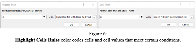
Finally, in row 26 is the Amount Over/Under Needs Maximum series. This calculation helps me keep track of how I’m doing with my spending on needs. In cell B26 is a simple formula that is subtracting my 50% for Needs from my Needs Total: =B24-B10. In this case, any negative amount in row 26 means that I am spending under the maximum. Conversely, a positive number means I’m spending over. To make this clear, I used Conditional Formatting in cell B26 (Figure 5).

This command is found in the Home tab > Styles group. I clicked on cell B26 then applied some formatting conditions:

1. Using Highlight Cells Rules > Greater Than… and Highlight Cells Rules > Less Than…, I formatted any amounts over the maximum to be displayed as red, while any amounts under the maximum are displayed as green (Figure 6). (Remember that a returned value of “$0.00” means that this part of your budget is perfectly balanced, so anything greater than “0” is over, and anything less than “0” is under.)
   
   
   
   
   
2. Using Icon Sets > More Rules, I formatted any amounts over the maximum to include an “up” arrow, while any amounts under the maximum include a “down” arrow (Figure 7).
   
   
   
   
   

Last but not least, I copied and pasted all of the data and formatting rules to the remaining cells in this section, C14:M26, once again using AutoFill (Figure 4).

Costs of Wants

In this section, I organized my data in the same way and used the same formatting rules as the previous section, Costs of Needs. The only difference here, of course, is that I am tracking the money I spend on things that are not essential. I also copied and pasted all of the data and formatting rules using AutoFill (Figure 4).

Savings Accrued

In this final section, I calculated the savings I’m left with after my expenses and whether that amount is at, above, or below 20% of my Total Net Monthly Income (B8). The Savings Total series subtracts Needs Total (B24) and Wants Total (B33) from Total Net Monthly Income (B8). That formula, in cell B37, looks like this: =B8-B24-B33. Keep in mind that this total includes retirement contributions and any/all extra payments made toward outstanding loan balances, so you may want to know how much of that savings total is liquid (i.e., going into a separate savings account where it can be withdrawn and used at any time). More on that in a moment.

The next two series, Actual Percentage of Net Monthly Income and Amount Over/Under Savings Minimum, work like their counterparts in Costs of Needs and Costs of Wants, but with one important difference. Since Amount Over/Under is calculating the amount over or under a minimum (as opposed to a maximum), I needed to subtract the 20% for Savings (B12) from my Savings Total (B37), which is the opposite of how these amounts were calculated for needs and wants totals. That formula, in cell B39, looks like this: =B37-B12.

Next, I wanted to know how much of my savings was liquid, which means that I had to subtract the savings earmarked for specific things. One of those things is Monthly Retirement Contribution. This particular amount, like Monthly Premiums in the Costs of Needs section, is automatically calculated by relative referencing. In cell B40 is the formula =B6. (If you make any changes to your monthly retirement contribution, be sure to make that change in cell B6, not B40.) I also added, as examples of other types of savings, the Extra Payment- Mortgage series and Extra Payment- Car Loan series. Remember, as I explained in the 50/30/20 Budget Rule above, any extra payments towards outstanding balances are considered payments from your savings. I then added one more series, Liquid Savings, the cells in which subtract the retirement contribution and extra payment amounts from Savings Total (B37). That formula, in cell B43, looks like this: =B37-(SUM(B40:B42)). Note: I nested the SUM function within the formula so that if needed, I could insert a new row between rows 40 and 42 to accommodate a new savings goal, which would then be added to the formula automatically.

Finally, as with the two previous sections, I copied and pasted all of the data and formatting rules to the remaining cells in this section, C37:M43, using AutoFill (Figure 4).

Try This Out in Our Upcoming Excel Class!

Want to try building this worksheet yourself? Register for our Build a Budget with Excel class, taking place Saturday, August 13, at 10:00 am. I will walk you through the steps of creating this worksheet so you can enhance your Excel skills and walk away with your own personal budgeting tool! (Basic Excel skills required.)

For Further Reading

Books for Adults

All Your Worth: The Ultimate Lifetime Money Plan
by Elizabeth Warren and Amelia Warren Tyagi

The book that pioneered the 50/30/20 rule. It contains very detailed definitions of must-haves, wants, and savings, so if you are unsure how to categorize one or more of your expenses, this no-nonsense book has you covered. It also offers several worksheets to help you break down your expenses and savings.

Financially Fearless: The LearnVest Program for Taking Control of Your Money
by Alexa Von Tobel

Von Tobel, a Certified Financial Planner and founder and managing partner of Inspired Capital, a venture capital firm, provides another straightforward book about using the 50/30/20 rule (or 50/20/30, as she calls it) to maintain a realistic budget. In this book, Von Tobel not only gives examples of common expenses, but assigns them allocated percentages within their respective categories. You’ll also find great tips for savings, such as creating an emergency fund (“Freedom Fund”) and saving for kids.

Books for Kids & Teens

Building Blocks of Finance (series)

The books in this charmingly illustrated finance series teach kids the ins and outs of spending, saving, investing, managing credit, and more!

First to a Million: A Teenager’s Guide to Achieving Early Financial Freedom
by Dan Sheeks

In this book, Dan Sheeks, owner and founder of SheeksFreaks LLC, teaches teens how to become financially independent, or what he calls “FI Freaks,” so that they can build the future they want. He also covers personal finance basics, like tracking income and expenses, and building a credit score.

TIP: Want to find all titles the Mercer County Library System has on personal finance? Type 332.024 into the catalog search bar. It will return all titles under the Dewey Decimal Classification for personal finance, estate planning, saving and thrift.

Online Database

Financial Ratings Series

My personal favorite among Mercer County Library System’s Business and Finance databases, Financial Ratings Series Online combines, in their words, “the strength of Weiss Ratings and Grey House Publishing to offer the library community a single source for Financial Strength Ratings and Financial Planning Tools covering Insurance, Medigap Plans, Banks, Credit Unions, Mutual Funds, Stocks, and Helpful Financial Literacy Tools to help users get started.”

Be sure to check out their Financial Literacy Tools, located in the main menu. There you will find a variety of downloadable guides covering all things personal finance, like buying a home, saving for your child’s education, and how to stick to a budget (yes, they endorse the 50/30/20 rule!).

To access the database outside the library, just follow the link above, then, from the homepage, click on the account icon in the top-right corner. You will then be prompted to enter your library card number.

- by Keith B., Technology Instruction